LipidSigR offers several utility functions to enhance convenience in constructing input SummarizedExperiment object, viewing output results, listing selectable lipid characteristics, and more.
Construct SE object
The input data for most functions must be a SummarizedExperiment
object, constructed by LipidSigR::as_summarized_experiment
or generated from other upstream analysis functions.
To begin analyzing data, follow the instructions below to construct the input SummarizedExperiment object. First, prepare the required input data frames: the abundance data and the group information table. If you only intend to conduct the profiling analysis, you only need to prepare the abundance data.
Prepare input data frames
The input abundance data and group information table must be provided as data frames and adhere to the following requirements.
Abundance data: The lipid abundance data includes the abundance values of each feature across all samples.
- The first column of abundance data must contain a list of lipid names (features).
- Each lipid name (feature) is unique.
- All abundance values are numeric.
For example:
rm(list = ls())
data("abundance_twoGroup")
head(abundance_twoGroup[, 1:6], 5)
#>      feature control_01 control_02 control_03 control_04 control_05
#> 1 Cer 38:1;2  0.1167960  0.1638070  0.1759450  0.1446540   0.172092
#> 2 Cer 40:1;2  0.7857833  0.9366095  0.8944465  0.8961396   1.056512
#> 3 Cer 40:2;2  0.1494030  0.1568970  0.1909800  0.1312440   0.248504
#> 4 Cer 42:1;2  1.8530153  2.1946591  2.6377576  2.3418783   2.143355
#> 5 Cer 42:2;2  1.3325520  1.2514943  1.9466750  1.2948319   1.634636
Group information table: The group information table contains the grouping details corresponding to the samples in lipid abundance data.
- For two-group data, column names must be arranged in order of
sample_name,label_name,group, andpair, and for multi-group data, column names must be arranged in order ofsample_name,label_name, andgroup. - All sample names are unique.
- Sample names in
sample_namecolumn are as same as the sample names in lipid abundance data. - Columns of
sample_name,label_name, andgroupcolumns do not contain NA values. - For two-group data, the column
groupcontain 2 groups, and for multi-group data the columngroupmust contain more than 2 groups. - In the ‘pair’ column for paired data, each pair must be sequentially numbered from 1 to N, ensuring no missing, blank, or skipped numbers are missing; otherwise, the value should be all marked as NA. (NOTE: The group information table of multi-group data should not contain this column.)
For example:
Mapping lipid characteristics
The purpose of this step is to exclude lipid features not recognized
by rgoslin::parseLipidNames.
If you haven’t install rgoslin package, install it by
running the following codes.
if (!require("BiocManager", quietly = TRUE))
    install.packages("BiocManager")

BiocManager::install("rgoslin")
Then, follow the instructions below before constructing the input data as a SummarizedExperiment object.
- In this step, an error message will be returned if
rgoslin::parseLipidNamescannot recognize a certain lipid. However, if your data contains at least two recognizable lipids, it will be sufficient for analysis (note that different analyses may have varying data requirements).
library(dplyr)
library(rgoslin)
# map lipid characteristics by rgoslin
parse_lipid <- rgoslin::parseLipidNames(lipidNames=abundance_twoGroup$feature)
#> Encountered an error while parsing 'SE 27:1;0-14:0;0': Expecting a single string value: [type=character; extent=4].
#> Encountered an error while parsing 'SE 27:1;0-15:0;0': Expecting a single string value: [type=character; extent=4].
#> Encountered an error while parsing 'SE 27:1;0-16:0;0': Expecting a single string value: [type=character; extent=4].
#> Encountered an error while parsing 'SE 27:1;0-16:1;0': Expecting a single string value: [type=character; extent=4].
#> Encountered an error while parsing 'SE 27:1;0-17:0;0': Expecting a single string value: [type=character; extent=4].
#> Encountered an error while parsing 'SE 27:1;0-17:1;0': Expecting a single string value: [type=character; extent=4].
#> Encountered an error while parsing 'SE 27:1;0-18:1;0': Expecting a single string value: [type=character; extent=4].
#> Encountered an error while parsing 'SE 27:1;0-18:2;0': Expecting a single string value: [type=character; extent=4].
#> Encountered an error while parsing 'SE 27:1;0-18:3;0': Expecting a single string value: [type=character; extent=4].
#> Encountered an error while parsing 'SE 27:1;0-19:2;0': Expecting a single string value: [type=character; extent=4].
#> Encountered an error while parsing 'SE 27:1;0-19:3;0': Expecting a single string value: [type=character; extent=4].
#> Encountered an error while parsing 'SE 27:1;0-20:2;0': Expecting a single string value: [type=character; extent=4].
#> Encountered an error while parsing 'SE 27:1;0-20:4;0': Expecting a single string value: [type=character; extent=4].
#> Encountered an error while parsing 'SE 27:1;0-20:5;0': Expecting a single string value: [type=character; extent=4].
#> Encountered an error while parsing 'SE 27:1;0-22:6;0': Expecting a single string value: [type=character; extent=4].
#> Encountered an error while parsing 'ST 27:1;0': Expecting a single string value: [type=character; extent=4].

# filter lipid recognized by rgoslin
recognized_lipid <- parse_lipid$Original.Name[
    which(parse_lipid$Grammar != 'NOT_PARSEABLE')]
abundance <- abundance_twoGroup %>%
    dplyr::filter(feature %in% recognized_lipid)
goslin_annotation <- parse_lipid %>%
    dplyr::filter(Original.Name %in% recognized_lipid)
After running the above code, two data frames,
abundance, and goslin_annotation, will be
generated and used in the next step.
head(abundance[, 1:6], 5)
#>      feature control_01 control_02 control_03 control_04 control_05
#> 1 Cer 38:1;2  0.1167960  0.1638070  0.1759450  0.1446540   0.172092
#> 2 Cer 40:1;2  0.7857833  0.9366095  0.8944465  0.8961396   1.056512
#> 3 Cer 40:2;2  0.1494030  0.1568970  0.1909800  0.1312440   0.248504
#> 4 Cer 42:1;2  1.8530153  2.1946591  2.6377576  2.3418783   2.143355
#> 5 Cer 42:2;2  1.3325520  1.2514943  1.9466750  1.2948319   1.634636
head(goslin_annotation[, 1:6], 5)
#>   Normalized.Name Original.Name Grammar Message Adduct Adduct.Charge
#> 1     Cer 38:1;O2    Cer 38:1;2  Goslin      NA     NA             0
#> 2     Cer 40:1;O2    Cer 40:1;2  Goslin      NA     NA             0
#> 3     Cer 40:2;O2    Cer 40:2;2  Goslin      NA     NA             0
#> 4     Cer 42:1;O2    Cer 42:1;2  Goslin      NA     NA             0
#> 5     Cer 42:2;O2    Cer 42:2;2  Goslin      NA     NA             0
Construct SE object
Use the data obtained from previous steps to construct SE object.
se <- as_summarized_experiment(
    abundance, goslin_annotation, group_info=group_info_twoGroup,
    se_type='de_two', paired_sample=FALSE)
#> Input data info
#> se_type: de_two
#> Number of lipids (features) available for analysis: 192
#> Number of samples: 23
#> Number of group: 2
#> Not paired samples.
After running the above code, you are ready to begin the analysis
with the output se. After the code execution, a summary of
the input data will be displayed.
(Note: If errors occur during execution, please revise the input data to resolve them.)
Extract data in SE object
Most of our statistical functions return results in a SummarizedExperiment object. To enhance user accessibility, we provide a function to extract these results as several data frames for easier viewing.
For example, after conducting LipidSigR::deSp_twoGroup,
it returns deSp_se. You can view the data stored in the
returned SummarizedExperiment object using
LipidSigR::extract_summarized_experiment.
# data processing
processed_se <- data_process(
    se, exclude_missing=TRUE, exclude_missing_pct=70,
    replace_na_method='min', replace_na_method_ref=0.5,
    normalization='Percentage')
# conduct differential expression analysis of lipid species
deSp_se <- deSp_twoGroup(
    processed_se, ref_group='ctrl', test='t-test',
    significant='pval', p_cutoff=0.05, FC_cutoff=1, transform='log10')
# extract results in SE
res_list <- extract_summarized_experiment(deSp_se)
# summary of extract results
summary(res_list)
#>                     Length Class      Mode
#> abundance           24     data.frame list
#> lipid_char_table    72     data.frame list
#> group_info           5     data.frame list
#> all_deSp_result     15     data.frame list
#> sig_deSp_result     15     data.frame list
#> processed_abundance 24     data.frame list
#> significant          1     -none-     character
#> p_cutoff             1     -none-     numeric
#> FC_cutoff            1     -none-     numeric
#> transform            1     -none-     character
The returned result list, extracted from the SummarizedExperiment object, includes input data (abundance, lipid characteristics table, group information table), various input settings (e.g., significance level, p-value cutoff), and statistical results.
Data processsing
Most input data for LipidSigR must undergo data
processing to ensure it is normalized without missing values. The data
processing function operates on the constructed SummarizedExperiment
object, processing the abundance table based on the user’s settings. The
resulting SummarizedExperiment object can then be used directly in
subsequent analysis functions.
# abundance in input SE
head(extract_summarized_experiment(se)$abundance[, 1:5], 10)
#>              feature control_01 control_02 control_03 control_04
#> 1         Cer 38:1;2  0.1167960  0.1638070  0.1759450  0.1446540
#> 2         Cer 40:1;2  0.7857833  0.9366095  0.8944465  0.8961396
#> 3         Cer 40:2;2  0.1494030  0.1568970  0.1909800  0.1312440
#> 4         Cer 42:1;2  1.8530153  2.1946591  2.6377576  2.3418783
#> 5         Cer 42:2;2  1.3325520  1.2514943  1.9466750  1.2948319
#> 6  DAG 14:0;0-18:1;0         NA  1.0664249         NA         NA
#> 7  DAG 16:0;0-16:0;0         NA         NA         NA         NA
#> 8  DAG 16:0;0-18:1;0  3.1378101  5.3820724  2.1217224  3.9616688
#> 9  DAG 16:0;0-18:2;0  2.1500685  2.1844099  0.9782799  4.7669999
#> 10 DAG 16:1;0-18:1;0  1.3524184  1.4611123  0.3797060  1.4499917

# data processing
processed_se <- data_process(
    se, exclude_missing=TRUE, exclude_missing_pct=70,
    replace_na_method='min', replace_na_method_ref=0.5,
    normalization='Percentage')

# abundance in processed SE
head(extract_summarized_experiment(processed_se)$abundance[, 1:5], 10)
#>              feature   control_01  control_02  control_03   control_04
#> 1         Cer 38:1;2 0.0041853183 0.005062099 0.006639506 0.0046739931
#> 2         Cer 40:1;2 0.0281580981 0.028943877 0.033753065 0.0289556495
#> 3         Cer 40:2;2 0.0053537717 0.004848560 0.007206871 0.0042406954
#> 4         Cer 42:1;2 0.0664017529 0.067821160 0.099539106 0.0756696884
#> 5         Cer 42:2;2 0.0477512444 0.038674706 0.073460234 0.0418380078
#> 6  DAG 16:0;0-18:1;0 0.1124416422 0.166321225 0.080065870 0.1280076083
#> 7  DAG 16:0;0-18:2;0 0.0770464839 0.067504429 0.036916625 0.1540290956
#> 8  DAG 16:1;0-18:1;0 0.0484631465 0.045152494 0.014328684 0.0468514603
#> 9  DAG 18:1;0-18:1;0 0.3812287315 0.345006230 0.147065473 0.2628932938
#> 10 DAG 18:2;0-18:0;0 0.0002579212 0.012558032 0.004138136 0.0002325649
After data processing, you can further visualize the differences by plotting the abundance before and after processing.
# plotting
data_process_plots <- plot_data_process(se, processed_se)

# result summary
summary(data_process_plots)
#>                                Length Class  Mode
#> interactive_boxPlot_before     8      plotly list
#> static_boxPlot_before          9      gg     list
#> interactive_densityPlot_before 8      plotly list
#> static_densityPlot_before      9      gg     list
#> interactive_boxPlot_after      8      plotly list
#> static_boxPlot_after           9      gg     list
#> interactive_densityPlot_after  8      plotly list
#> static_densityPlot_after       9      gg     list

# view box plot before/after data processing
data_process_plots$static_boxPlot_before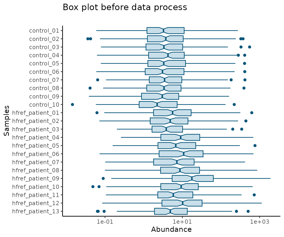
data_process_plots$static_boxPlot_after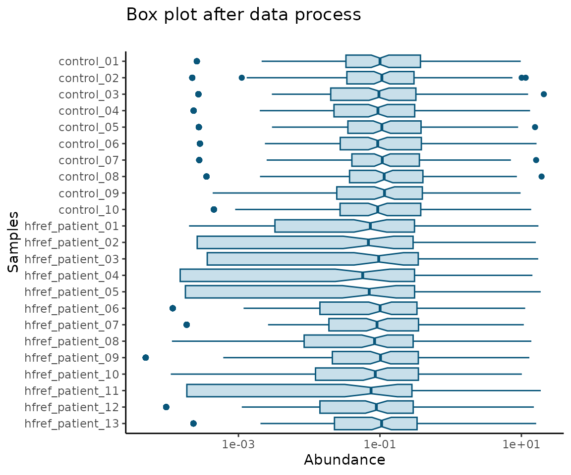
# view density plot before/after data processing
data_process_plots$static_densityPlot_before 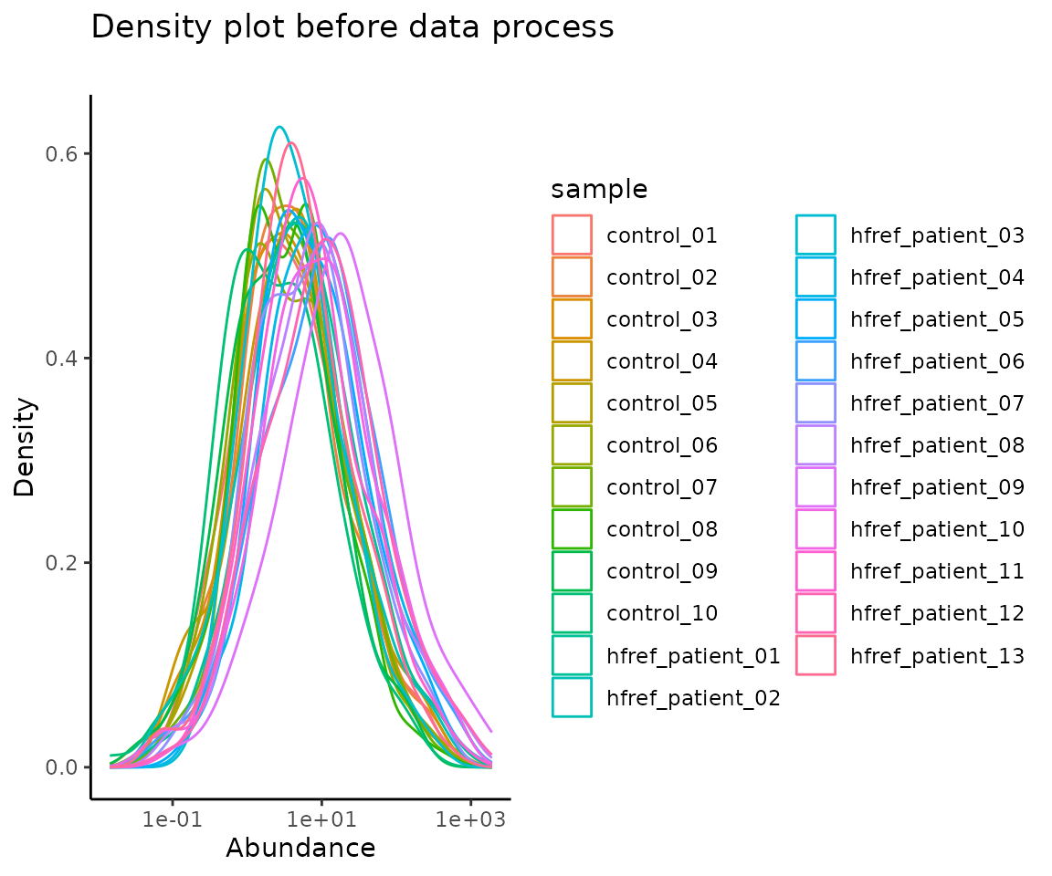
data_process_plots$static_densityPlot_after 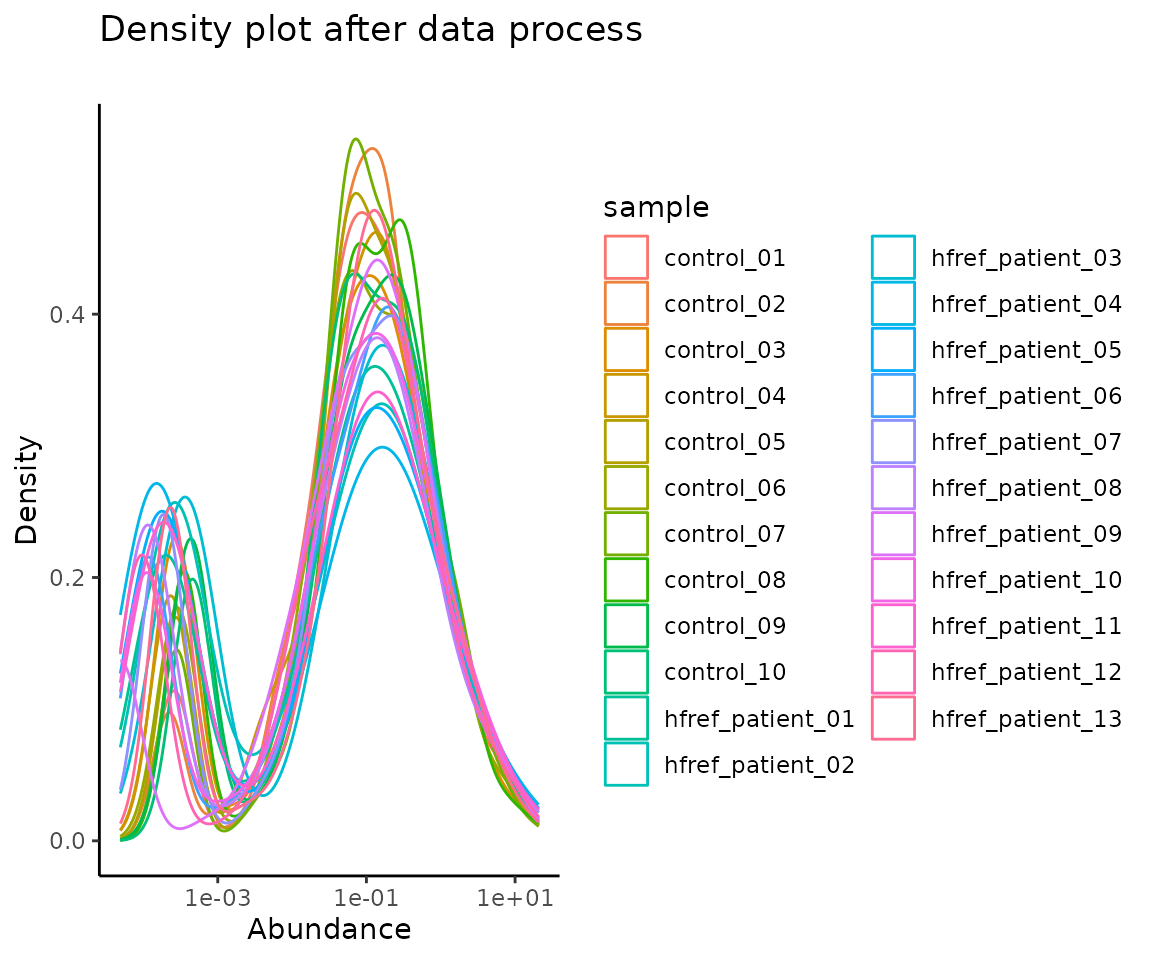
Obtain lipid characteristics
In several functions, you must select a specific lipid characteristic
as input for analysis. To enhance accessibility, we provide the
LipidSigR::list_lipid_char function, which returns all
available lipid characteristics. You can review these options and choose
one as your input.
LipidSigR::list_lipid_char returns three types of lipid
characteristic lists: deChar_list,
chain_db_list, and common_list, each used in
different analyses.
deChar_list: the selectable lipid characteristics for using
LipidSigR::deChar_twoGroupandLipidSigR::deChar_multiGroup.chain_db_list: the selectable lipid characteristics for using
LipidSigR::heatmap_chain_db.ml_char_list: the selectable lipid characteristics for using
LipidSigR::ml_model.common_list: the selectable lipid characteristics for use in all functions not mentioned above.
Take LipidSigR::lipid_profiling as an example.
# data processing
processed_se <- data_process(
    se, exclude_missing=TRUE, exclude_missing_pct=70,
    replace_na_method='min', replace_na_method_ref=0.5,
    normalization='Percentage')

# get lipid characteristics
list_lipid_char(processed_se)$common_list
#> There are 4 ratio characteristics that can be converted in your dataset.
#>            Lipid classification            Lipid classification
#>                      "Category"                    "Main.Class"
#>            Lipid classification            Lipid classification
#>                     "Sub.Class"                         "class"
#>           Fatty acid properties           Fatty acid properties
#>                            "FA"                          "FA.C"
#>           Fatty acid properties           Fatty acid properties
#>     "FA.Chain.Length.Category1"     "FA.Chain.Length.Category2"
#>           Fatty acid properties           Fatty acid properties
#>     "FA.Chain.Length.Category3"                         "FA.DB"
#>           Fatty acid properties           Fatty acid properties
#>                         "FA.OH"     "FA.Unsaturation.Category1"
#>           Fatty acid properties           Fatty acid properties
#>     "FA.Unsaturation.Category2"                       "Total.C"
#>           Fatty acid properties           Fatty acid properties
#>                      "Total.DB"                      "Total.FA"
#>           Fatty acid properties Physical or chemical properties
#>                      "Total.OH"             "Bilayer.Thickness"
#> Physical or chemical properties Physical or chemical properties
#>                     "Bond.type"              "Headgroup.Charge"
#> Physical or chemical properties Physical or chemical properties
#>           "Intrinsic.Curvature"             "Lateral.Diffusion"
#> Physical or chemical properties              Cellular component
#>        "Transition.Temperature"            "Cellular.Component"
#>                        Function
#>                      "Function"

# conduct lipid profiling function
result <- lipid_profiling(processed_se, char="class")
#> There are 4 ratio characteristics that can be converted in your dataset.
Lipid annotation
“Mapping lipid characteristics” is one of the steps in constructing
the input SummarizedExperiment object in LipidSigR,
detailed in previous section.
When the Goslin annotation table is provided to the
LipidSigR::as_summarized_experiment, it is extended into a
lipid characteristic table by adding mappings between lipids, the LION
ontology, and other resource IDs. This extended lipid characteristic
table is then included in the returned SE object. If you only need the
lipid characteristic table, you can use this
LipidSigR::lipid_annotation directly.
# the input lipid annotation table
head(goslin_annotation[, 1:6], 5)
#>   Normalized.Name Original.Name Grammar Message Adduct Adduct.Charge
#> 1     Cer 38:1;O2    Cer 38:1;2  Goslin      NA     NA             0
#> 2     Cer 40:1;O2    Cer 40:1;2  Goslin      NA     NA             0
#> 3     Cer 40:2;O2    Cer 40:2;2  Goslin      NA     NA             0
#> 4     Cer 42:1;O2    Cer 42:1;2  Goslin      NA     NA             0
#> 5     Cer 42:2;O2    Cer 42:2;2  Goslin      NA     NA             0

# conduct lipid annotation
lipid_annotation_table <- lipid_annotation(goslin_annotation)

# view lipid annotation table
head(lipid_annotation_table[, 1:5], 5)
#>      feature class Lipid.Maps.Category Species.Name Molecular.Species.Name
#> 1 Cer 38:1;2   Cer                  SP  Cer 38:1;O2                   <NA>
#> 2 Cer 40:1;2   Cer                  SP  Cer 40:1;O2                   <NA>
#> 3 Cer 40:2;2   Cer                  SP  Cer 40:2;O2                   <NA>
#> 4 Cer 42:1;2   Cer                  SP  Cer 42:1;O2                   <NA>
#> 5 Cer 42:2;2   Cer                  SP  Cer 42:2;O2                   <NA>

# columns of returned lipid annotation table
colnames(lipid_annotation_table)
#>  [1] "feature"                   "class"
#>  [3] "Lipid.Maps.Category"       "Species.Name"
#>  [5] "Molecular.Species.Name"    "Structural.Species.Name"
#>  [7] "Level"                     "Mass"
#>  [9] "Sum.Formula"               "Total.FA"
#> [11] "Total.C"                   "Total.DB"
#> [13] "Total.OH"                  "FA"
#> [15] "FA.C"                      "FA.DB"
#> [17] "FA.OH"                     "LCB"
#> [19] "LCB2"                      "LCB.C"
#> [21] "LCB.DB"                    "LCB.OH"
#> [23] "LCB.Bond.Type"             "FA1"
#> [25] "FA1.C"                     "FA1.DB"
#> [27] "FA1.OH"                    "FA1.Bond.Type"
#> [29] "FA2"                       "FA2.C"
#> [31] "FA2.DB"                    "FA2.OH"
#> [33] "FA2.Bond.Type"             "FA3"
#> [35] "FA3.C"                     "FA3.DB"
#> [37] "FA3.OH"                    "FA3.Bond.Type"
#> [39] "FA4"                       "FA4.C"
#> [41] "FA4.DB"                    "FA4.OH"
#> [43] "FA4.Bond.Type"             "Category"
#> [45] "Main.Class"                "Sub.Class"
#> [47] "Cellular.Component"        "Function"
#> [49] "Bond.type"                 "Headgroup.Charge"
#> [51] "Lateral.Diffusion"         "Bilayer.Thickness"
#> [53] "Intrinsic.Curvature"       "Transition.Temperature"
#> [55] "FA.Unsaturation.Category1" "FA.Unsaturation.Category2"
#> [57] "FA.Chain.Length.Category1" "FA.Chain.Length.Category2"
#> [59] "FA.Chain.Length.Category3" "LION.abbr"
#> [61] "GATOM.abbr"                "LIPIDMAPS.reaction.abbr"
#> [63] "LION.ID"                   "LIPID.MAPS.ID"
#> [65] "SwissLipids.ID"            "HMDB.ID"
#> [67] "ChEBI.ID"                  "KEGG.ID"
#> [69] "LipidBank.ID"              "PubChem.CID"
#> [71] "MetaNetX.ID"               "PlantFA.ID"
Lipid species abundance conversion
Two conversion types for lipid species are provided: summing lipid species abundance by lipid characteristics or converting to ratio-based abundance.
Both functions are integrated into the lipid characteristics analysis
function, so when you use LipidSigR::deChar_twoGroup or
LipidSigR::deChar_multiGroup, the abundance conversion is
automatically performed within the function.
If you only want to obtain the converted abundance, follow the commands below.
- NOTE: The input data must be a SummarizedExperiment object
constructed using
LipidSigR::as_summarized_experimentand then further processed withLipidSigR::data_process. Please readvignette("1_tool_function")before preparing the input data.
Convert from species to characteristics
# view input abundance
head(extract_summarized_experiment(processed_se)$abundance[, 1:5], 5)
#>      feature  control_01  control_02  control_03  control_04
#> 1 Cer 38:1;2 0.004185318 0.005062099 0.006639506 0.004673993
#> 2 Cer 40:1;2 0.028158098 0.028943877 0.033753065 0.028955649
#> 3 Cer 40:2;2 0.005353772 0.004848560 0.007206871 0.004240695
#> 4 Cer 42:1;2 0.066401753 0.067821160 0.099539106 0.075669688
#> 5 Cer 42:2;2 0.047751244 0.038674706 0.073460234 0.041838008

# convert species abundance to characteristic abundance
char_abundance <- convert_sp2char(processed_se, transform='log10')

# view abundance after conversion
head(extract_summarized_experiment(char_abundance)$abundance[, 1:5], 5)
#>     feature  control_01   control_02 control_03  control_04
#> 1 class|Cer -0.81858467 -0.837583766 -0.6563969 -0.80861038
#> 2  class|DG  0.03385835 -0.008210876 -0.3062842  0.08584996
#> 3 class|LPC  0.53341062  0.281360639  0.4567495  0.23801049
#> 4 class|LPE -0.79973292 -1.089284167 -0.7307483 -1.00166907
#> 5  class|PC  1.67965445  1.680565780  1.8237574  1.71690075
Convert from species to ratio
# view input abundance
head(extract_summarized_experiment(processed_se)$abundance[, 1:3], 5)
#>      feature  control_01  control_02
#> 1 Cer 38:1;2 0.004185318 0.005062099
#> 2 Cer 40:1;2 0.028158098 0.028943877
#> 3 Cer 40:2;2 0.005353772 0.004848560
#> 4 Cer 42:1;2 0.066401753 0.067821160
#> 5 Cer 42:2;2 0.047751244 0.038674706

# convert species abundance to characteristic abundance
ratio_abundance <- convert_sp2ratio(processed_se, transform='log2')
#> There are 4 ratio characteristics that can be converted in your dataset.

# view abundance after conversion
head(extract_summarized_experiment(ratio_abundance )$abundance[, 1:3], 5)
#>                                              feature  control_01   control_02
#> 1                 Chains Ether/Ester linked ratio|PC -4.53128351 -4.579168367
#> 2                 Chains Ether/Ester linked ratio|PE  0.04700296 -0.008048668
#> 3                           Chains odd/even ratio|PC -4.64947013 -4.635198329
#> 4                        Chains odd/even ratio|PC O- -9.75844582 -9.634882752
#> 5 Ratio of Lysophospholipids to Phospholipids|LPL/PL -3.85431934 -4.703840948