“Correlation” provides functions such as correlation coefficients and linear regression to analyze continuous clinical features correlating with lipid species or characteristics.
All of the input data of functions must be a SummarizedExperiment
object constructed by LipidSigR::as_summarized_experiment.
For detailed instructions for constructing SummarizedExperiment object,
please read vignette("1_tool_function").
- NOTE: Some functions will require
processed_se, which is the SummarizedExperiment object after being processed byLipidSigR::data_process. Please readvignette("1_tool_function").
To use our data as an example, follow the steps below.
# load package
library(LipidSigR)

# load the example SummarizedExperiment
data("corr_data")

# data processing
processed_se <- data_process(
    corr_data, exclude_missing=TRUE, exclude_missing_pct=70,
    replace_na_method='min', replace_na_method_ref=0.5,
    normalization='Percentage')
Correlation analysis can be performed on either “lipid species” or “lipid characteristics”.
- Lipid Species Analysis: Data is analyzed at the individual lipid species level.
- Lipid Characteristics Analysis: Data is aggregated by specific lipid characteristics. The abundance of all lipid species in the same categories of a selected characteristic is summed up for analysis.
This section is designed for continuous clinical data. The
condition_col parameter specifies the column name from the
group information table that defines the clinical conditions for
analysis. Please ensure the selected columns contain only numerical data
(e.g., integers, floats). NOTE: The condition_col must include at
least two clinical conditions.
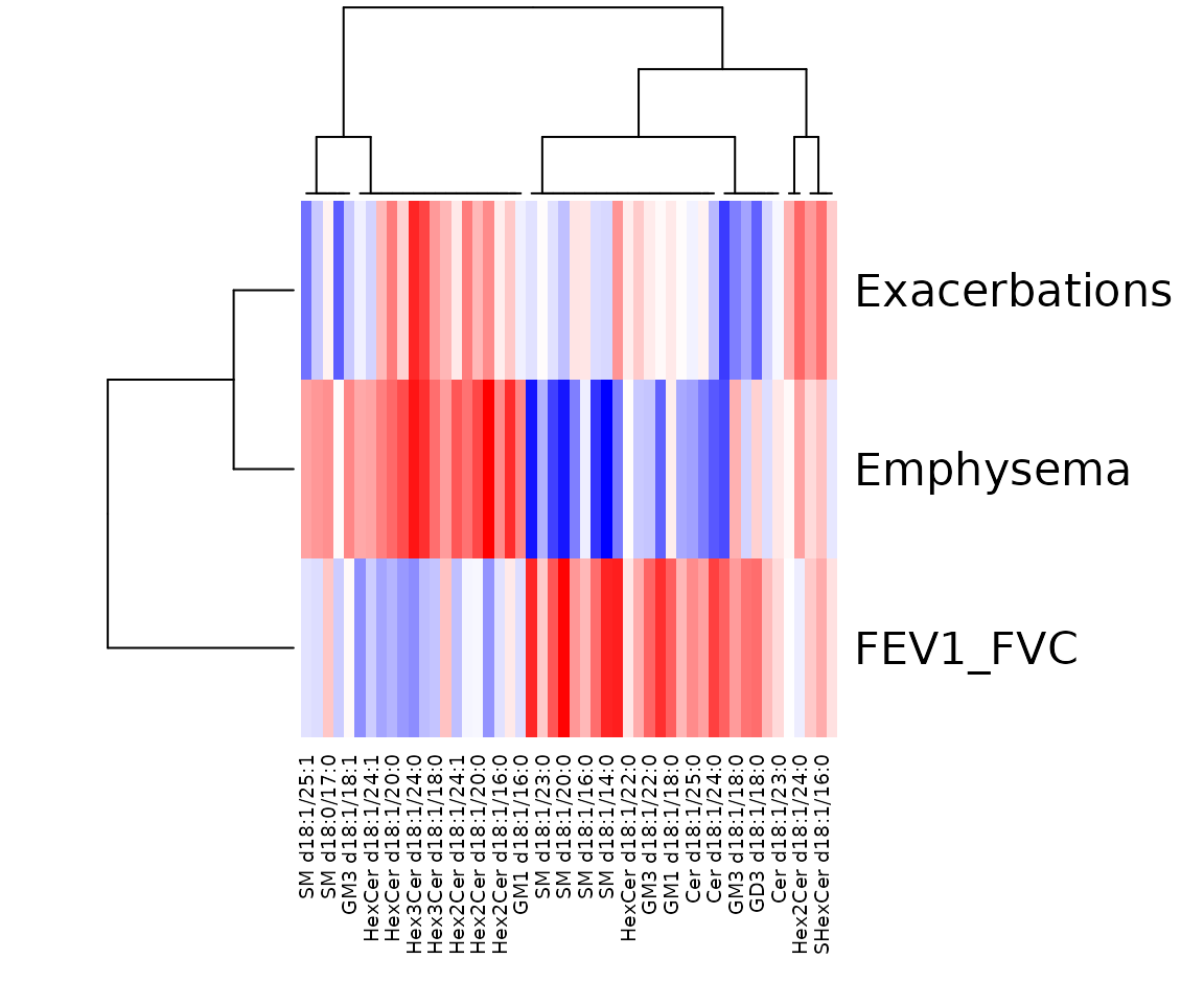
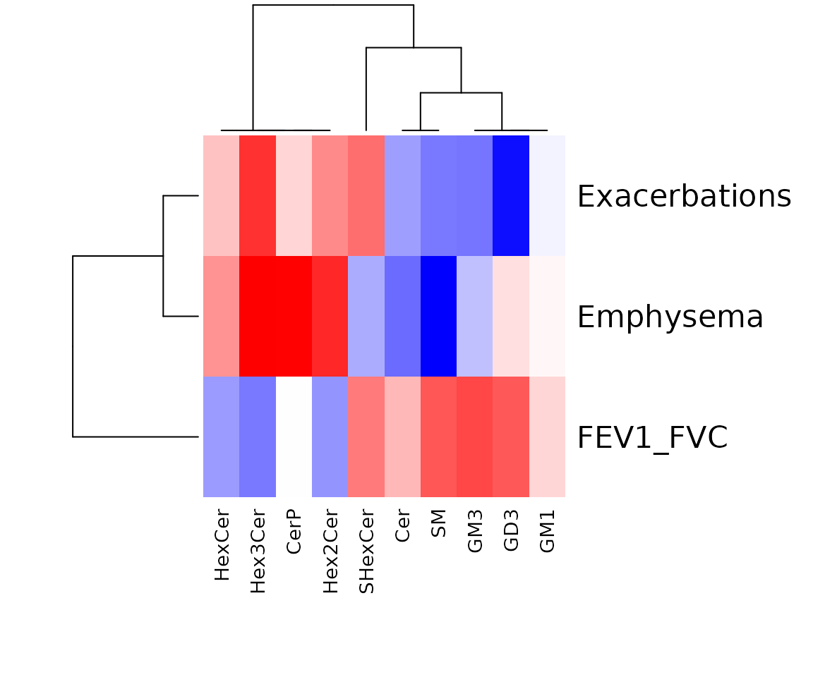
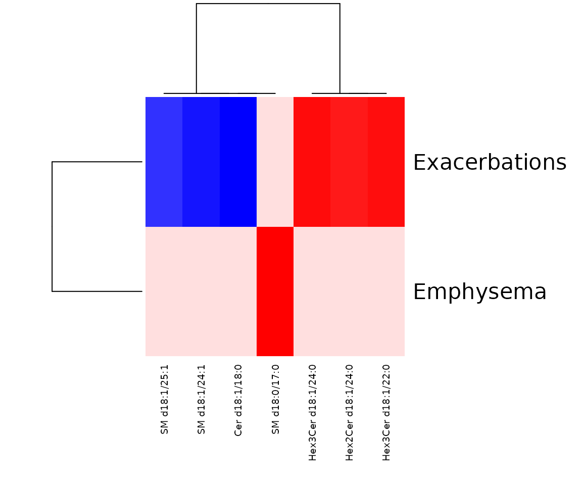
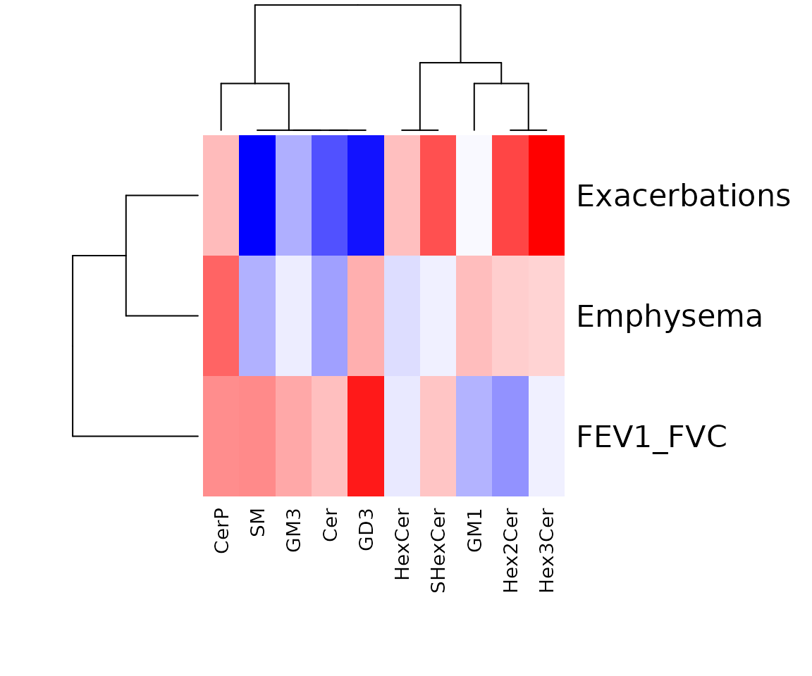
Two correlation analyses are accessible: ‘Correlation Coefficient’ and ‘Linear Regression’. Heatmaps will be shown once the correlation analysis is completed, it depicts the pattern between lipid species/lipid characteristics and clinical features.
The available clustering methods are as follows.
- Distance measurement: Pearson, Spearman, Kendall, Euclidean, Maximum, Manhattan, Canberra, Binary, and Minkowski.
- Clustering method: median, average, single, complete, Ward.D, Ward.D2, WPGMA, and UPGMC.
Correlation coefficient
The Correlation Coefficient gives a summary view of whether a
relationship exists between clinical features and lipid species, how
strong that relationship is, and whether the relationship is positive or
negative. The parameters’ cor_coef_cutoff and
p_cutoff can decide the correlation coefficient and p-value
cut-offs. The rule of thumb in medical research recommended by Mukaka
for interpreting the size of a correlation coefficient is provided below
(Mukaka 2012).
| Size of Correlation | Interpretation |
|---|---|
| 0.90 to 1.00 (-.90 to -1.00) | Very high positive (negative) correlation |
| 0.70 to .90 (-.70 to -.90) | High positive (negative) correlation |
| 0.50 to .70 (-.50 to -.70) | Moderate positive (negative) correlation |
| 0.30 to .50 (-.30 to -.50) | Low positive (negative) correlation |
| 0.00 to .30 (.00 to -.30) | negligible correlation |
Before the analysis, we must determine the condition_col
parameter, selected from the column names from the group information
table. Follow the steps below to view all available options for
condition_col.
# extract group information table
group_info <- extract_summarized_experiment(processed_se)$group_info

# condition_col options (choose only columns with numeric values)
condition_col_option <- str(group_info[-1])
#> 'data.frame':    129 obs. of  8 variables:
#>  $ FEV1_FVC     : num  0.29 0.57 0.79 0.39 0.37 0.41 0.79 0.58 0.39 0.48 ...
#>  $ Emphysema    : num  11.017 2.361 0.983 34.993 26.85 ...
#>  $ Exacerbations: num  6 0 0 0 0 0 5 0 0 0 ...
#>  $ Age          : num  48.7 70.1 49.6 54.1 70.5 58.8 71.5 69.5 72.2 69.3 ...
#>  $ Sex          : num  0 0 0 1 0 1 0 0 1 1 ...
#>  $ Smoking      : num  0 0 0 0 0 0 0 0 1 0 ...
#>  $ BMI          : num  36.5 27.9 23.9 28.4 23.2 ...
#>  $ FEV1         : num  14.9 66.7 99.9 31.2 31.6 57.7 98.1 54.3 44.4 46.3 ...
Lipid species correlation
For lipid species correlation analysis, set the type
parameter to Sp. Optionally, you can visualize the heatmap
with side colors by specifying a characteristic in the
side_color_char parameter (e.g., ‘class’). You can view all
available characteristics from the common list returned by
LipidSigR::list_lipid_char. If you prefer not to display
side colors, set side_color_char to NULL.
NOTE: The char parameter must be set to NULL for
lipid species correlation.
# compute correlation coefficient and visualize by heatmap
res_sp <- corr_cor_heatmap(
    processed_se, char=NULL,
    condition_col=c("FEV1_FVC", "Emphysema", "Exacerbations"),
    side_color_char='class', correlation='pearson', significant='pval',
    p_cutoff=1, adjust_p_method='BH', cor_coef_cutoff=0,
    distfun='spearman', hclustfun='average', heatmap_col='statistic',
    transform='log10', type='Sp')

# result summary
summary(res_sp)
#>                        Length Class        Mode
#> all_correlation_result   9    data.frame   list
#> sig_correlation_result   9    data.frame   list
#> interactive_heatmap      8    plotly       list
#> static_heatmap           3    recordedplot list
#> heatmap_matrix         150    -none-       numeric
# view result: heatmap of clinical features and lipid species
res_sp$static_heatmap
Correlation coefficient for lipid species analysis The heatmap shows only the variables that pass the defined cut-offs for the p-value and the correlation coefficient. The rows are clinical features, and the columns are the lipid species.
Lipid characteristics correlation
For lipid characteristics analysis, set the type parameter to
Char and specify a lipid characteristic in the char
parameter (e.g., ‘class’). Use LipidSigR::list_lipid_char
to view the available lipid characteristics. For more detailed
information, please refer to
vignette("1_tool_function").
NOTE: The side_color_char parameter must be set to
NULL for lipid characteristics correlation.
# compute correlation coefficient and visualize by heatmap
res_char <- corr_cor_heatmap(
    processed_se, char="class",
    condition_col=c("FEV1_FVC", "Emphysema", "Exacerbations"),
    side_color_char=NULL, correlation='pearson', significant='pval',
    p_cutoff=1, adjust_p_method='BH', cor_coef_cutoff=0,
    distfun='spearman', hclustfun='average', heatmap_col='statistic',
    transform='log10', type='Char')

# result summary
summary(res_char)
#>                        Length Class        Mode
#> all_correlation_result  9     data.frame   list
#> sig_correlation_result  9     data.frame   list
#> interactive_heatmap     8     plotly       list
#> static_heatmap          3     recordedplot list
#> heatmap_matrix         30     -none-       numeric
# view result: heatmap of clinical features and lipid characteristics
res_char$static_heatmap
Correlation coefficient for lipid characteristics analysis The heatmap shows only the variables that pass the defined cut-offs for the p-value and the correlation coefficient. The rows are clinical features, and the columns are lipid characteristics.
Linear regression
Linear regression is a statistical method used to model the relationship between a dependent variable (e.g., lipid level) and one or more independent variables (e.g., clinical features). By analyzing these relationships, we can estimate the impact of specific clinical factors on lipid levels.
In multiple linear regression, we incorporate additional variables to
account for potential confounding factors. To do this, we specify the
adjusted_col parameter, which refers to the column names
selected from the group information table. Once the analysis is
complete, each lipid species is assigned a beta coefficient and a
corresponding t-statistic (p-value). These values can be used to
identify significant associations and group similar lipid species for
further analysis.
Before the analysis, we must determine the condition_col
and adjusted_col parameters, selected from the column names
from the group information table. Follow the steps below to view all
available options for condition_col and
adjusted_col.
# extract group information table
group_info <- extract_summarized_experiment(processed_se)$group_info

# condition_col options (choose only columns with numeric values)
condition_col_option <- str(group_info[-1])
#> 'data.frame':    129 obs. of  8 variables:
#>  $ FEV1_FVC     : num  0.29 0.57 0.79 0.39 0.37 0.41 0.79 0.58 0.39 0.48 ...
#>  $ Emphysema    : num  11.017 2.361 0.983 34.993 26.85 ...
#>  $ Exacerbations: num  6 0 0 0 0 0 5 0 0 0 ...
#>  $ Age          : num  48.7 70.1 49.6 54.1 70.5 58.8 71.5 69.5 72.2 69.3 ...
#>  $ Sex          : num  0 0 0 1 0 1 0 0 1 1 ...
#>  $ Smoking      : num  0 0 0 0 0 0 0 0 1 0 ...
#>  $ BMI          : num  36.5 27.9 23.9 28.4 23.2 ...
#>  $ FEV1         : num  14.9 66.7 99.9 31.2 31.6 57.7 98.1 54.3 44.4 46.3 ...

# adjusted_col options
adjusted_col_option <- str(group_info[-1])
#> 'data.frame':    129 obs. of  8 variables:
#>  $ FEV1_FVC     : num  0.29 0.57 0.79 0.39 0.37 0.41 0.79 0.58 0.39 0.48 ...
#>  $ Emphysema    : num  11.017 2.361 0.983 34.993 26.85 ...
#>  $ Exacerbations: num  6 0 0 0 0 0 5 0 0 0 ...
#>  $ Age          : num  48.7 70.1 49.6 54.1 70.5 58.8 71.5 69.5 72.2 69.3 ...
#>  $ Sex          : num  0 0 0 1 0 1 0 0 1 1 ...
#>  $ Smoking      : num  0 0 0 0 0 0 0 0 1 0 ...
#>  $ BMI          : num  36.5 27.9 23.9 28.4 23.2 ...
#>  $ FEV1         : num  14.9 66.7 99.9 31.2 31.6 57.7 98.1 54.3 44.4 46.3 ...
Lipid species correlation
For lipid species correlation analysis, set the type
parameter to Sp. Optionally, you can visualize the heatmap
with side colors by specifying a characteristic in the
side_color_char parameter (e.g., ‘class’). You can view all
available characteristics from the common list returned by
LipidSigR::list_lipid_char. If you prefer not to display
side colors, set side_color_char to NULL.
NOTE: The char parameter must be set to NULL for
lipid species correlation.
# compute linear regression and visualize by heatmap
res_sp <- corr_lr_heatmap(
    processed_se, char=NULL,
    condition_col=c("FEV1_FVC", "Emphysema", "Exacerbations"),
    adjusted_col=c("Age", "Sex", "Smoking", "BMI", "FEV1"),
    side_color_char=NULL, significant='pval', p_cutoff=0.05,
    adjust_p_method='BH', distfun='spearman', hclustfun='centroid',
    heatmap_col='t_statistic', transform='log10', type='Sp')

# result summary
summary(res_sp)
#>                        Length Class        Mode
#> all_correlation_result  9     data.frame   list
#> sig_correlation_result  9     data.frame   list
#> interactive_heatmap     8     plotly       list
#> static_heatmap          3     recordedplot list
#> heatmap_matrix         14     -none-       numeric
# view result: heatmap of linear regression
res_sp$static_heatmap
The heatmap of linear regression for lipid species analysis The heatmap shows only the variables that pass the user-defined cut-offs for p-value and correlation coefficient. The rows are clinical features, and the columns are lipid species.
Lipid characteristics correlation
For lipid characteristics correlation, set the type
parameter to Char and specify a lipid characteristic for
the char parameter. You can use
LipidSigR::list_lipid_char to view a list of available
lipid characteristics. For more detailed information, please refer to
vignette("1_tool_function").
NOTE: The side_color_char parameter must be set to
NULL for lipid characteristics correlation.
# compute linear regression and visualize by heatmap
res_char <- corr_lr_heatmap(
    processed_se, char="class",
    condition_col=c("FEV1_FVC", "Emphysema", "Exacerbations"),
    adjusted_col=c("Age", "Sex", "Smoking", "BMI", "FEV1"),
    side_color_char=NULL, significant='pval', p_cutoff=1,
    adjust_p_method='BH', distfun='spearman', hclustfun='centroid',
    heatmap_col='t_statistic', transform='log10', type='Char')

# result summary
summary(res_char)
#>                        Length Class        Mode
#> all_correlation_result  9     data.frame   list
#> sig_correlation_result  9     data.frame   list
#> interactive_heatmap     8     plotly       list
#> static_heatmap          3     recordedplot list
#> heatmap_matrix         30     -none-       numeric
# view result: heatmap of linear regression
res_char$static_heatmap
The heatmap of linear regression for lipid characteristics analysis Only the variables that pass the user-defined cut-offs for p-value and correlation coefficient are shown on the heatmap. The rows of the heatmap are clinical features, and the columns are lipid characteristics.