Enrichment analysis provides two main approaches: ‘Over Representation Analysis (ORA)’ and ‘Lipid Set Enrichment Analysis (LSEA)’. ORA analysis illustrates significant lipid species enriched in the categories of lipid class. LSEA analysis is a computational method determining whether an a priori-defined set of lipids shows statistically significant, concordant differences between two biological states (e.g., phenotypes).
The input data must be a SummarizedExperiment object
deSp_se generated by LipidSigR::deSp_twoGroup
or LipidSigR::deSp_multiGroup. Please read
lipid species differential expression analysis section in
vignette("de").
To use our data as an example, follow the steps below.
# load package
library(LipidSigR)

# load the example SummarizedExperiment
data("de_data_twoGroup")

# data processing
processed_se <- data_process(
    de_data_twoGroup, exclude_missing=TRUE, exclude_missing_pct=70,
    replace_na_method='min', replace_na_method_ref=0.5,
    normalization='Percentage', transform='log10')

# conduct differential expression analysis of lipid species
deSp_se <- deSp_twoGroup(
    processed_se, ref_group='ctrl', test='t-test',
    significant='pval', p_cutoff=0.05, FC_cutoff=1, transform='log10')
Over Representation Analysis (ORA)
The Over-Representation analysis provides whether significant lipid species are enriched in the categories of lipid class. Results are presented in tables and bar plots categorizing lipid species into ‘up-regulated’ or ‘down-regulated’ groups based on log2 fold change.
Here, we use two-group data as an example.
# conduct ORA
ora_all <- enrichment_ora(
    deSp_se, char=NULL, significant='pval', p_cutoff=0.05)

# result summary
summary(ora_all)
#>                     Length Class      Mode
#> enrich_result       14     tbl_df     list
#> static_barPlot      11     gg         list
#> interactive_barPlot  8     plotly     list
#> table_barPlot       10     grouped_df list

# view result: ORA bar plot
ora_all$static_barPlot 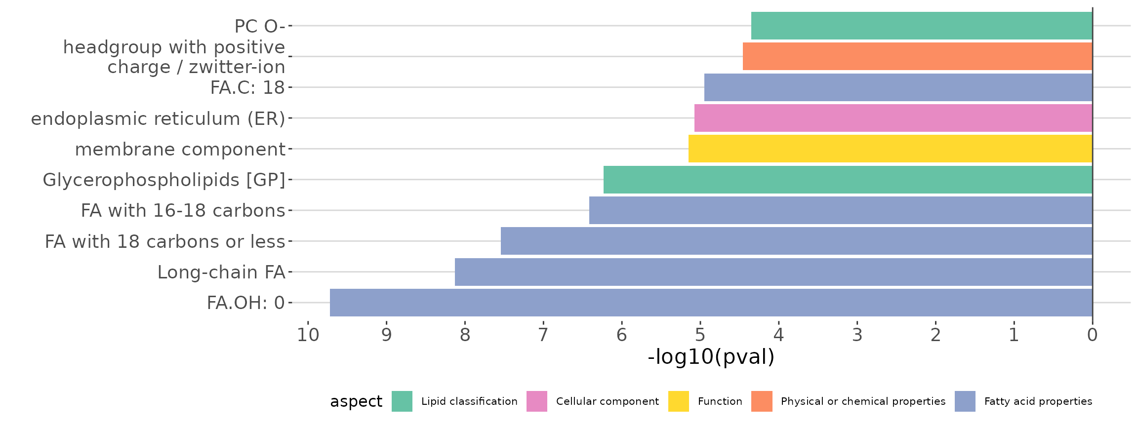
ORA bar plot of all characteristics The bar plot shows the top 10 significant up-regulated and down-regulated terms.
- You can obtain the selectable lipid characteristics for the
charinput usingLipidSigR::list_lipid_char. Please readvignette("tool_function").
Here, we use class as the char input for an
example.
# conduct ORA of a specific `char`
ora_one <- enrichment_ora(
    deSp_se, char='class', significant='pval', p_cutoff=0.05)

# result summary
summary(ora_one)
#>                     Length Class      Mode
#> enrich_result       14     tbl_df     list
#> static_barPlot      11     gg         list
#> interactive_barPlot  8     plotly     list
#> table_barPlot       11     grouped_df list

# view result: ORA bar plot
ora_one$static_barPlot 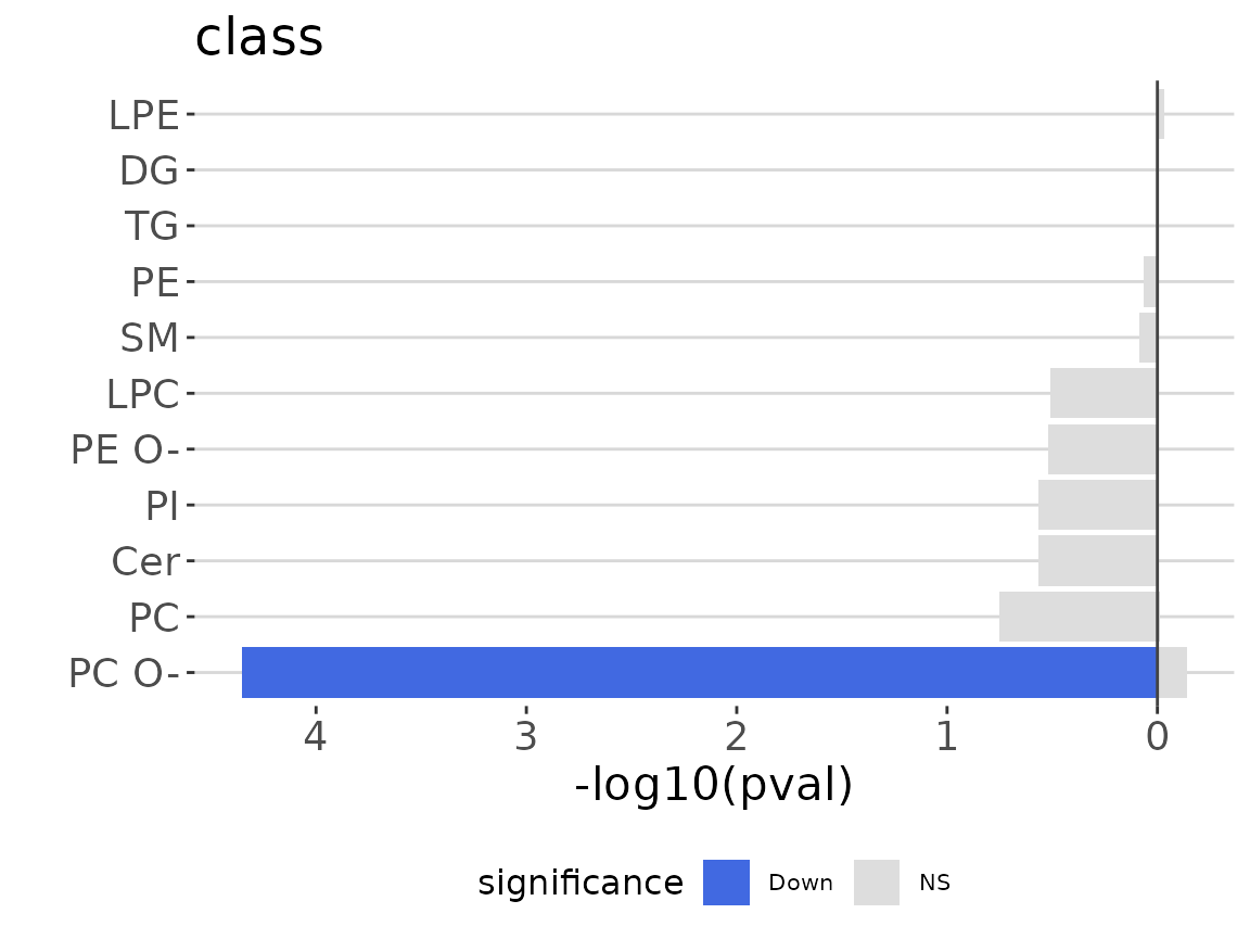
ORA bar plot of specific characteristics The bar plot classifies significant lipid species into ‘up-regulated’ or ‘down-regulated’ categories based on their log2 fold change, according to a selected characteristic. Red bars indicate up-regulated, blue bars represent down-regulated, and grey bars signify non-significant.
Lipid Set Enrichment Analysis (LSEA)
Lipid Set Enrichment Analysis (LSEA) is a computational method determining whether an a priori-defined set of lipids shows statistically significant, concordant differences between two biological states (e.g., phenotypes). Results are presented in tables and bar plots categorizing lipid species into ‘up-regulated’ or ‘down-regulated’ groups based on NES (Normalized Enrichment Score), and a table.
# conduct LSEA
lsea_all <- enrichment_lsea(
    deSp_se, char=NULL, rank_by='statistic', significant='pval',
    p_cutoff=0.05)

# result summary
summary(lsea_all)
#>                     Length Class  Mode
#> enrich_result        11    tbl_df list
#> static_barPlot       11    gg     list
#> interactive_barPlot   8    plotly list
#> table_barPlot         8    tbl_df list
#> lipid_set           167    -none- list
#> ranked_list         182    -none- numeric

# view result: LSEA bar plot
lsea_all$static_barPlot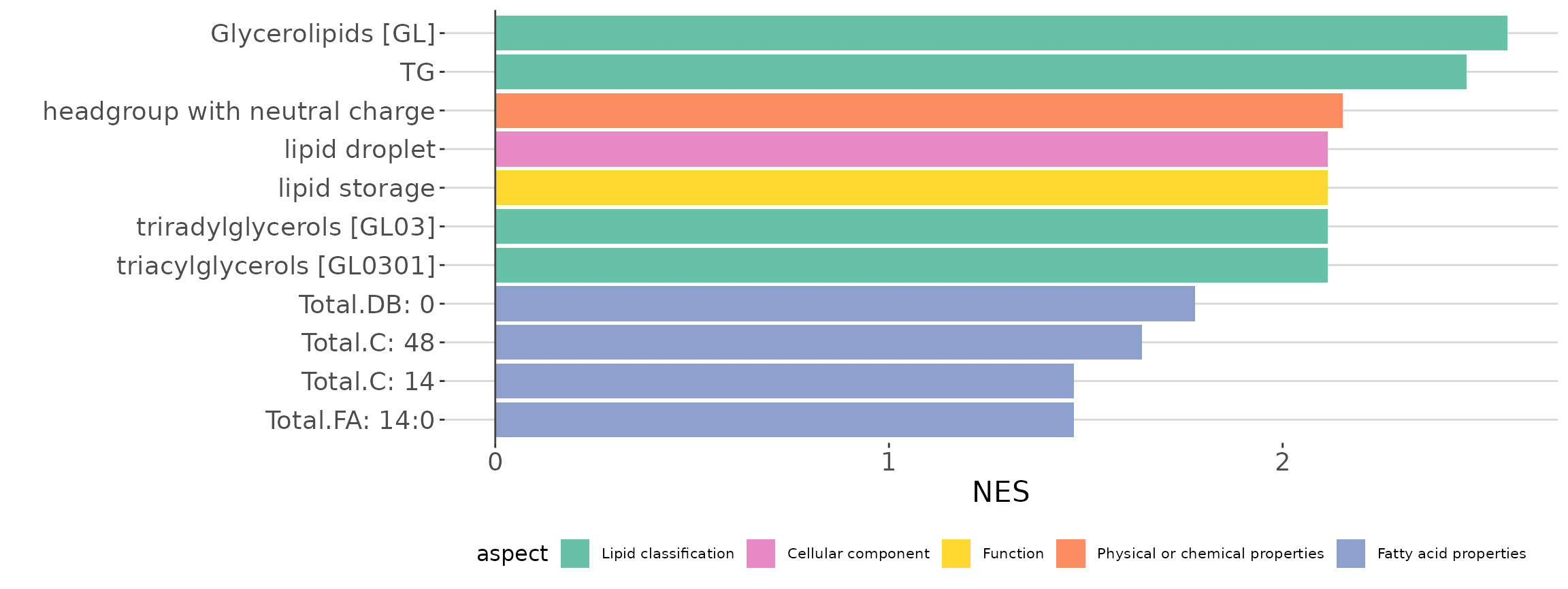
LSEA bar plot of all characteristics The bar plot shows the top 10 significant up-regulated and down-regulated terms.
- You can obtain the selectable lipid characteristics for the
charinput usingLipidSigR::list_lipid_char. Please readvignette("tool_function").
Here, we use class as the char input for an
example.
# conduct LSEA of a specific `char`
lsea_one <- enrichment_lsea(
    deSp_se, char='class', rank_by='statistic',
    significant='pval', p_cutoff=0.05)

# result summary
summary(lsea_one)
#>                     Length Class  Mode
#> enrich_result        11    tbl_df list
#> static_barPlot       11    gg     list
#> interactive_barPlot   8    plotly list
#> table_barPlot         9    tbl_df list
#> lipid_set            11    -none- list
#> ranked_list         182    -none- numeric

# view result: LSEA bar plot
lsea_one$static_barPlot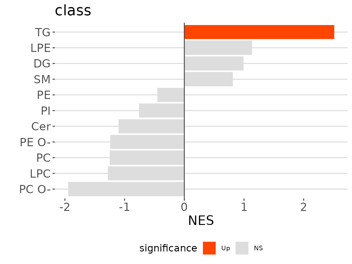
LSEA bar plot of a specific char The
bar plot classifies significant lipid species into ‘up-regulated’ or
‘down-regulated’ categories based on their log2 fold change, according
to a selected characteristic. Red bars indicate up-regulated, blue bars
represent down-regulated, and grey bars signify non-significant.
After running enrichment_lsea, you can continue
executing plot_enrichment_lsea to plot the enrichment plot
further. Please use the whole output of enrichment_lsea as
the input for plotting.
# plot LSEA results
lsea_plot <- plot_enrichment_lsea(
    lsea_res=lsea_one, char='class', char_feature='TG')

# view result: enrichment plot
lsea_plot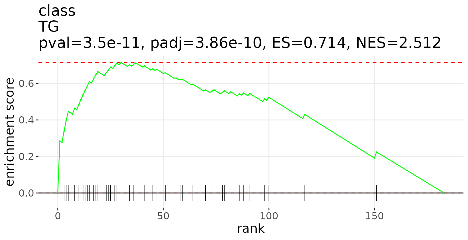
Session info
#> R version 4.4.3 (2025-02-28)
#> Platform: x86_64-pc-linux-gnu
#> Running under: CentOS Stream 9
#>
#> Matrix products: default
#> BLAS/LAPACK: FlexiBLAS OPENBLAS-OPENMP;  LAPACK version 3.9.0
#>
#> locale:
#>  [1] LC_CTYPE=en_US.UTF-8       LC_NUMERIC=C
#>  [3] LC_TIME=en_US.UTF-8        LC_COLLATE=en_US.UTF-8
#>  [5] LC_MONETARY=en_US.UTF-8    LC_MESSAGES=en_US.UTF-8
#>  [7] LC_PAPER=en_US.UTF-8       LC_NAME=C
#>  [9] LC_ADDRESS=C               LC_TELEPHONE=C
#> [11] LC_MEASUREMENT=en_US.UTF-8 LC_IDENTIFICATION=C
#>
#> time zone: Asia/Taipei
#> tzcode source: system (glibc)
#>
#> attached base packages:
#> [1] stats4    stats     graphics  grDevices utils     datasets  methods
#> [8] base
#>
#> other attached packages:
#>  [1] SummarizedExperiment_1.36.0 Biobase_2.66.0
#>  [3] GenomicRanges_1.58.0        GenomeInfoDb_1.42.3
#>  [5] IRanges_2.40.1              S4Vectors_0.44.0
#>  [7] BiocGenerics_0.52.0         MatrixGenerics_1.18.1
#>  [9] matrixStats_1.5.0           LipidSigR_1.0.2
#> [11] dplyr_1.1.4
#>
#> loaded via a namespace (and not attached):
#>  [1] fastmatch_1.1-6         gtable_0.3.6            xfun_0.52
#>  [4] bslib_0.9.0             ggplot2_3.5.2           htmlwidgets_1.6.4
#>  [7] lattice_0.22-7          crosstalk_1.2.1         vctrs_0.6.5
#> [10] tools_4.4.3             generics_0.1.3          parallel_4.4.3
#> [13] tibble_3.2.1            pkgconfig_2.0.3         Matrix_1.7-3
#> [16] data.table_1.17.0       RColorBrewer_1.1-3      desc_1.4.3
#> [19] lifecycle_1.0.4         GenomeInfoDbData_1.2.13 compiler_4.4.3
#> [22] farver_2.1.2            stringr_1.5.1           textshaping_1.0.0
#> [25] fgsea_1.32.4            codetools_0.2-20        htmltools_0.5.8.1
#> [28] sass_0.4.10             lazyeval_0.2.2          yaml_2.3.10
#> [31] plotly_4.10.4           pillar_1.10.2           pkgdown_2.1.2
#> [34] crayon_1.5.3            jquerylib_0.1.4         tidyr_1.3.1
#> [37] BiocParallel_1.40.2     cachem_1.1.0            DelayedArray_0.32.0
#> [40] abind_1.4-8             tidyselect_1.2.1        digest_0.6.37
#> [43] stringi_1.8.7           purrr_1.0.4             labeling_0.4.3
#> [46] ggthemes_5.1.0          cowplot_1.1.3           fastmap_1.2.0
#> [49] grid_4.4.3              cli_3.6.5               SparseArray_1.6.2
#> [52] magrittr_2.0.3          S4Arrays_1.6.0          withr_3.0.2
#> [55] UCSC.utils_1.2.0        scales_1.4.0            rmarkdown_2.29
#> [58] XVector_0.46.0          httr_1.4.7              ragg_1.4.0
#> [61] evaluate_1.0.3          knitr_1.50              viridisLite_0.4.2
#> [64] rlang_1.1.6             Rcpp_1.0.14             glue_1.8.0
#> [67] rgoslin_1.10.0          rstudioapi_0.17.1       jsonlite_2.0.0
#> [70] R6_2.6.1                systemfonts_1.2.2       fs_1.6.6
#> [73] zlibbioc_1.52.0